ML 4: Kit & Kaboodle
- Published on
- ∘ 182 min read ∘ ––– views
Index
- Index
- Introduction
- Chapter 1: The Reinforcement Learning Problem
- Chapter 2: Multi-arm Bandits
- Chapter 3: Finite Markov Decision Processes
- Chapter 4: Dynamic Programming
- Chapter 5: Monte Carlo Methods
- 5.1 Monte Carlo Prediction
- 5.2 Monte Carlo Estimation of Action Values
- 5.3 Monte Carlo Control
- 5.4 Monte Carlo Control Without Exploring Starts
- 5.5 Off-policy Prediction via Importance Sampling
- 5.6 Incremental Implementation
- 5.7 Off-Policy Monte Carlo Control
- 5.8 Importance Sampling on Truncated Returns
- 5.9 Summary
- Chapter 6 Temporal-Difference Learning
- Chapter 7: Eligibility Traces
- Chapter 8: Planning and Learning with Tabular Methods
Introduction
Notes from Sutton & Barto's "Reinforcement Learning: an Introduction".
Glossary
"Capital letters are used for random variables and major algorithm variables. Lower case letters are used for the values of random variables and for scalar functions. Quantities that are required to be real-valued vectors are written in bold and in lower case (even if random variables)."
| Variable | Meaning |
|---|---|
| state | |
| action | |
| set of all nonterminal states | |
| set of all states, including the terminal state | |
| set of possible in state | |
| set of possible rewards | |
| discrete time step | |
| final time step of an episode | |
| state at | |
| action at | |
| reward at , dependent, like , on and | |
| return (cumulative discounted reward) following | |
| -step return | |
| -step return | |
| policy, decision-making rule | |
| the optimal policy | |
| action take in state under policy | |
| probability of taking action in state under policy | |
| probability of transition to state , with reward from | |
| value of state under policy (expected return) | |
| value of state under the optimal policy | |
| value of taking action in state under policy | |
| value of taking action in state the optimal policy | |
| estimate (a random variable) of or | |
| estimate (a random variable) of or | |
| approximate value of state given a vector of weights | |
| approximate value of a state-action par given weights | |
| vector of (possibly learned) underlying an approximate value function | |
| vector of features visible when in state | |
| inner product of vectors , e.g. | |
| temporal-difference error at (a random variable, even though not upper case) | |
| eligibility trace for state at | |
| eligibility trace for a state-action pair | |
| eligibility trace vector at | |
| discount rate parameter | |
| probability of random action in -greedy policy | |
| step-size parameters | |
| decay-rate parameter for eligibility traces |
Chapter 1: The Reinforcement Learning Problem
1.1 Reinforcement Learning
Reinforcement learning is different from supervised learning, the kind of learning studied in most current research in the field of machine learning. Supervised learning is learning from a training set of labeled examples provided by a knowledgable external supervisor. Each example is a description of a situation together with a specification—the label—of the correct action the system should take to that situation, which is often to identify a category to which the situation belongs. The object of this kind of learning is for the system to extrapolate, or generalize, its responses so that it acts correctly in situations not present in the training set.
Whereas reinforcement learning relies on interaction between an agent and the environment, supervised learning which utilizes the "omniscient" training data set.
Although one might be tempted to think of reinforcement learning as a kind of unsupervised learning because it does not rely on examples of correct behavior, reinforcement learning is trying to maximize a reward signal instead of trying to find hidden structure.
Reinforcement learning exists outside the dual paradigms of supervision in part due to the inherent trade-off between exploration and exploitation. In order to discover optimal actions (exploration), the agent must forego performing known actions and risk taking an unknown action.
The agent has to exploit what it already knows in order to obtain reward, but it also has to explore in order to make better action selections in the future
1.2 Examples
- A gazelle calf struggles to its feet minutes after being born. Half an hour later it is running at 20 miles per hour.
In all of the examples given, the agent's actions affect the future state of the environment in an unknown, but predictable way.
Correct choice requires taking into account indirect, delayed consequences of actions, and thus may require foresight or planning.
1.3 Elements of Reinforcement Learning
Reinforcement learning can be categorized by four main sub-elements (with main elements of agent, environment):
policy - defines the agent's behavior. Can be considered as a mapping from perceived states of the environment to actions to be taken when in those states.
reqard signal - defines the goal of the RL problem as the agent's purpose is to maximize reward
value function - whereas the reward signal indicates what is good in an immediate sense, a value function specifies what is good in the long run by accounting for the reward gained from states that are likely to follow from an action.
model of environment - mimics the behavior of the environment, allowing inferences to be made about how the environment will behave.
model-based - methods that rely on models (duh) and planning
model-free - explicit trial-and-error learners --> anti-planning
1.4 Limitations and Scope
While this book focuses on value-estimate functions as a core component of the algorithms discussed, alternative methods such as genetic algorithms and programming, simulated annealing, and other optimization methods have proven to be successful as well.
If action spaces are sufficiently small, or good policies are common, then these evolutionary approaches can be effective. However, methods that can exploit the details of individual behavioral interactions can be more efficient than the evolutionary methods listed above.
Some methods do not appeal to value functions, but merely search the policy spaces defined by a collection of numerical parameters, estimating the directions they need to tuned towards to most rapidly improve a policy's performance. Policy gradients like this have proven useful in many cases.
1.5 An Extended Example Tic-Tac-Toe
Consider a game of tic-tac-toe against an imperfect player whose play is sometimes incorrect and allows us to win. Whereas classical game theory techniques such as minimax offer solutions to intelligent/perfect opponents, they may fail in situations where they were not already disposed to win.
Classical optimization methods for sequential decision problems, such as dynamic programming, can compute an optimal solution for any opponent, but require as input a complete specification of that opponent, including the probabilities with which the opponent makes each move in each board state
An RL approach using a value function might make use of a table of numbers associated with each possible state in the game. Each number will be the latest estimate of the state's value, and the whole tabled is the learned value function. State A is said to be better than state B if the current estimate of the probability of our winning from A is higher than it is from B.
Assuming we always play Xs, then for all states with three Xs in a row the probability of winning is 1, because we have already won. Similarly, for all states with three Os in a row, or that are “filled up,” the correct probability is 0, as we cannot win from them. We set the initial values of all the other states to 0.5, representing a guess that we have a 50% chance of winning.
We play many games against the opponent. To select our moves we examine the states that would result from each of our possible moves (one for each blank space on the board) and look up their current values in the table. Most of the time we move greedily, selecting the move that leads to the state with greatest value, that is, with the highest estimated probability of winning. Occasionally, however, we select randomly from among the other moves instead. These are called exploratory moves because they cause us to experience states that we might otherwise never see.
Throughout the "playing" process, we update the values of the states we actually encounter from their initialized value of 0.5 in order to make our value estimates more accurate. To do this, we back up the current value of the earlier state to be closer to the value of the later state:
If the step-size parameter is reduced properly over time, this method converges, for any fixed opponent. If the step-size parameter is not reduced all the way to zero over time, then the agent also plays well against opponents that slowly change their strategy.
Evolutionary methods struggle to retain association between which actions caused positive reward, equally weighting all actions that contributed to a "win". In contrast, value functions evaluate individual states. Although both methods search the policy space, learning the value function takes advantage of the information available.
By adding a neural network to the tabular representation of the value-function, the agent can generalize from it's experiences so that it selects action based on information from similar stated experienced in the past. Here, supervised learning methods can help out, although neural nets are neither the only or best way to transcend tabularization.
The tic-tac-toe example agent is model-free in this sense w.r.t its opponent: it has no model of its opponent. However, this can be advantageous as it avoids complex method in which bottlenecks arise from constructing a sufficiently accurate environment model.
1.6 Summary
RL is the first field to seriously address the computational issues that arise when learning from interaction in order to achiever long-term goals. RL's use of value functions distinguishes reinforcement learning methods from evolutionary methods that search directly in policy space guided by scalar evaluations of entire policies.
Chapter 2: Multi-arm Bandits
RL is an evaluation oriented approach which retroactively improves rather than proactively instruct. Evaluative feedback depends on the actions taken, and instructive feedback is independent of the action. To study the evaluative aspect, we will work in a non-associative setting which reduces the complexity of the RL problem to highlight the former topic: the n-armed bandit problem.
2.1 An -Armed Bandit Problem
When repeatedly faced with different actions, after which the agent is rewarded from a stationary action-dependent probability distribution, how should you maximize expected total reward over some time period, say 1,000 time-steps. Each action has an estimated expected reward, called the value of that action.
If the agent prioritizes the action associated with the highest estimated value, this is called a greedy action resulting from exploiting the current knowledge of action-value pairs.
Choosing a non-greedy action for the sake of broadening exploitable knowledge is called exploration.
Exploitation is the right thing to do to maximize the expected reward on the one step, but exploration may produce the greater total reward in the long run ... Reward is lower in the short run, during exploration, but higher in the long run because after you have discovered the better actions, you can exploit them many times.
2.2 Action-Value Methods
In this chapter, the true value of action is denoted , and the estimated value on the -th time-step is . An intuitive estimation is the average rewards actually received when an action has been selection.
In other words, if by the -th time step action a has been chosen times prior to , yielding rewards , then its value is estimated to be
Note that as which is called the sample-average method for estimating action values as each estimate is the simple average o the sample of relevant rewards.
The simplest action selection rule is to select the action (or one of the actions) with highest estimated action value, that is, to select at step one of the greedy actions, , for which . This greedy action selection method can be written as
Greedy action selection always exploits current knowledge to maximize immediate reward spending no time sampling inferior actions. One solution to the exploration-exploitation conflict is -greedy exploration which is taking a random action with small probability instead of the exploitative action. -greedy methods are advantageous as, since each action has equal probability of being randomly selected, each action will be sampled an infinite number of times, guaranteeing s.t. converges to
Tests against an arbitrary 10-armed-bandit problem show that is a good general hyper parameter for -greedy exploration with trade offs between optimal-action discovery sooner vs better long-term performance.
It is also possible to reduce over time to try to get the best of both high and low values.
2.3 Incremental Implementation
The problem with the straightforward estimation of the value of an action as described in 2.1 is that it become memory and computationally intensive without bound over time. Each additional reward following an action requires more memory to store in order to determine . To fix, let denote the estimate for an agent's -th reward, that is the average of its first rewards. The average of all rewards is given by:
which only requires memory for , and minimally computation for each new reward.
The update rule is a form that occurs frequently throughout this textbook (foreshadowing the Bellman) whose general form is:
The is reduced by taking steps towards the which indicates a desirable direction to move, e.g. the -th reward. Note that the used in the incremental method above changes from time-step to time-step according the the parameter
2.4 Tracking a Nonstationary Problem
In cases where the environment is non-stationary and the "bandit" is changing over time, it makes sense to weight recent rewards more heavily than long-past ones. By using a constant step-size parameter, and modifying the incremental update rule from 2.3, we can achieve this effect:
where is constant s.t. is a weighted average of past rewards and the initial estimate :
This is the weighted average sum where . Note that because of exponential, recency-weighted average, if , then all the weight goes to the last reward.
Sometimes it is convenient to vary the step-size parameter from step to step. Let denote the step-size parameter used to process the reward received after the -th selection of action , where is the sample-average method which is guaranteed to converge to the true action values. But, convergence is not guaranteed for all choices of the sequence . Per stochastic approximation theory, the conditions to assure convergence with probability 1 are given by:
and
The first condition guarantees that steps are large enough to eventually overcome any initial conditions or random fluctuations and the second guarantees that they eventually become small enough to assure convergence. Note that both conditions are met for the sample-average case, but not for the case of constant step-size parameter.
2.5 Optimistic Initial Values
All the methods discussed above are to some degree dependent on or biased towards the initial action-value estimates . For sample-average methods, the bias disappears once all action have been selected at least once, but constant- methods retain permanent bias. Optimistic initial action values encourage exploration as most actions perform worse than the initial value, causing exploitative actions to attempt the other faux optimistic actions before beginning true exploration. At first, these methods tend to perform worse as they are more exploratory, but rapidly perform better as the need for exploration is resolved sooner.
However, such and approach is not effective in nonstationary problems as the drive for exploration is inherently temporary.
If the task changes, creating a renewed need for exploration, this method cannot help ... The beginning of time occurs only once, and thus we should not focus on it too much.
2.6 Upper-Confidence-Bound Action Selection
Exploration is needed while estimates of action values are uncertain. -greedy action selection force non-actions to be tried indiscriminately, with no preference for those that are nearly greedy or particularly uncertain.
It would be better to select among the non-greedy actions according to their potential for actually being optimal, taking into account both how close their estimates are to being maximal and the uncertainties in those estimates. One effective way of doing this is to select actions as:
where controls the degree of exploration and for , is considered a maximizing action.
The idea of this upper confidence bound (UCB) action selection is that the square-root term is a measure of the uncertainty or variance in the estimate of ’s value. Therefore, the quantity being 'ed over is a sort of upper bound on the possible true value of action , with the parameter determining the confidence level. Each time is selected, the uncertainty is presumably reduced; is incremented, and the term is square root decreased.
Another difficulty is dealing with large state spaces, ... In these more advanced settings there is currently no known practical way of utilizing the idea of UCB action selection.
2.7 Gradient Bandits
Another approach is learning a numerical preference for each . While the preference indicates the frequency of an action being taken, it has no interpretation in terms of reward. Only relative preference of one action over another is considered e.g. if we add an arbitrary, but equal amount to all the preferences, there is no affect on the action probabilities which are determine according to a soft-max (or Gibbs, Boltzmann) distribution:
, where initially, all preferences are the same () so that all action have an initial equal probability of being selected.
The application in stochastic gradient ascent is, after selecting the action and receiving reward , the preferences are updated by:
and
,
where is the step-size param, and is the average of all the rewards up through and including which can be computed incrementally (2.3, 2.4 for stationary and nonstationary problems, respectively). is the benchmark reward against which each reward is compared. The probability of taking is increased/decreased relative to it's difference with the benchmark. Non-selected actions move in the opposite direction.
Deeper insight can be gained by understanding it as a stochastic approximation to gradient ascent. In exact gradient ascent, each preference would be incrementing proportional to the increments effect on performance:
where the measure of the performance here is the expected reward:
While it's not possible it implement gradient ascent exactly as we do not know the , the updates using the preference updates are equal to the above equation in expected value, making the algorithm an instance of stochastic gradient ascent. This can be observed by:
where can be any scalar independent of . Here, the gradient sums to zero over all the actions:
As varies, some actions' probabilities go up, others down, s.t. the net change = 0 as the sum of the probabilities must remain equal to 1:
which is now in the form of an expectation summed over all possible values of the random variable :
where we've chosen and substituted for , which is permitted as and all other factors are non random. Shortly we'll establish that where
Which means that we now have:
With the intention of writing the performance gradient as an expectation of something that can be sampled at each step, and the updated on each step proportional to the sample, we can substitute the above expectation for the performance gradient which yields:
which is equivalent to the original algorithm.
After proving that , then we can show that the expected update of the gradient-bandit algorithm is equal to the gradient of the expected reward, and thus the algorithm is an instance of stochastic gradient ascent which in turn assures robust convergence properties.
Note that this is independent of the selected action ... The choice of the baseline does not affect the expected update of the algorithm, but it does affect the variance of the update and thus the rate of convergence
2.8 Associative Search (Contextual Bandits)
When there are different actions that need to be associated with different situation, a policy –that is, a mapping from situations to the actions that are best in those situations– needs to be learned.
Suppose there are several different -armed bandit tasks and that on each play one of these different tasks is confronted at random. Unless you randomly select the true action value for the given task, this method will. Suppose, however, that when the bandit task is selected against your agent, you are given a distinct clue about its identity (but, importantly, not its action values).
2.9 Summary
- ε-greedy methods choose randomly a small fraction of the time,
- UCB methods choose deterministically but achieve exploration by subtly favoring at each step the actions that have so far received fewer samples.
- Gradient-bandit algorithms estimate not action values, but action preferences, and favor the more preferred actions in a graded, probabilistic manner using a soft-max distribution.
The simple expedient of initializing estimates optimistically causes even greedy methods to explore significantly.
While UCB appears to perform best in the -bandit scenario, also note that each of the algorithms are fairly insensitive to their relevant hyperparemeters. Further sophisticated means of balancing the exploration-exploitation conflict are discussed here.
Chapter 3: Finite Markov Decision Processes
This chapter broadly characterizes the RL problem, presenting the idealized mathematical representation therein. Gathering insights from the mathematical structure, they introduce discussion of value functions and Bellman equations.
3.1 The Agent-Environment Interface
The learner and decision-maker is called the agent. The thing it interacts with, comprising everything outside the agent, is called the environment. These interact continually, the agent selecting actions and the environment responding to those actions and presenting new situations to the agent.
The agent interacts with the environment at each of the the discrete time steps, , with the agent receiving some representation of the environment's state , where is the set of possible states, and on that basis selects an action , where is the set of actions available in state . After each action is taken (that is, 1 time step later), the agent receives reward , and enters .
At each step, the agent develops its mapping from states to probabilities of selection each available action called it's policy , (where ), which represents a flexible and abstract framework that can be applied to a wide range of problems.
the boundary between agent and environment is not often the same as the physical boundary of a robot’s or animal’s body. Usually, the boundary is drawn closer to the agent than that ... The general rule we follow is that anything that cannot be changed arbitrarily by the agent is considered to be outside of it and thus part of its environment.
3.2 Goals and Rewards
In RL, the goal of the agent is formalized in terms of the reward function, where it attempts to maximize cumulative reward in the long run. It it critical to model success in such a way that indicates what we want to be accomplished: what not how. Rewards are computed in/by the environment, not the agent. This is important to maintain imperfect control so that the agent has to meaningfully interact with the environment rather than simply confer reward upon itself.
3.3 Returns
How do we formalize cumulative reward for maximization? If the sequence of rewards awarded after time step is denoted , then we can maximize the expected return , where is the final time step. This works for environments with terminal states at the end of each episode followed by a reset to a standard starting state.
In episodic tasks we sometimes need to distinguish the set of all non-terminal states, denoted , from the set of all states plus the terminal state, denoted .
In some cases, agent-environment interaction is not episodically divided; rather it is continuous and without limit. In these cases, it's unsuitable to use as presented above as , and return itself could be infinite (e.g. cart-pole). To fix this issue, we use discounting so that the agent tries to maximize the sum of discounted rewards ad-infinitum:
where , and is called the discount rate.
Gamma controls how near/farsighted the agent is.
If , the infinite sum has a finite value as long as the reward sequence is bounded. If , the agent is “myopic” in being concerned only with maximizing immediate rewards: its objective in this case is to learn how to choose so as to maximize only .
3.4 Unified Notation for Episodic and Continuing Tasks
refer to the the representation of a variable at time of episode . Additionally, the sum over a finite and infinite number of terms can be unified by considering the terminal step to be an absorbing state which transition only to itself and generates zero reward.
So, which includes the possibility of or , but not both.
3.5 The Markov Property
Certainly the state signal should include immediate sensations such as sensory measurements, but it can contain much more than that. State representations can be highly processed versions of original sensations, or they can be complex structures built up over time from the sequence of sensations ... On the other hand, the state signal should not be expected to inform the agent of everything about the environment, or even everything that would be useful to it in making decisions.
A state signal that succeeds in retaining all relevant information is said to be Markov, meaning that it summarizes everything about the complete sequence of positions (transition dynamics: SARSA) that led to it.
In the most general, discrete case, the necessary response may depend on everything that has happened earlier and can be defined as the complete probability distribution:
If a state signal is Markov, i.e. the environment's response depends only on the state and action representations of the current time step, then the dynamics can be defined by: . This, in turn, allows the agent to predict all future states and expected rewards from merely the given state.
Even if a state is non-Markov, it is useful to treat it as such, as the current state is always the fundamental basis for predicting future rewards which influence action selection.
The inability to have access to a perfect Markov state representation is probably not a severe problem for a reinforcement learning agent.
3.6 Markov Decision Processes
An RL task that satisfies the Markov property is called an MDP. If the state and action spaces are finite, then it is call a finite MDP.
Given the dynamics specified by , the agent can computer anything else it needs to know about the environment:
- Expected rewards for state-action pairs:
,
- State-transition probabilities:
- Expected reward for the state-action-next triples:
3.7 Value Functions
A Value function estimates how good it is to be in a given state, or how good it is to perform a given action in a given state, defined in terms of expected reward. The value of a state under a policy : , is the expected return when starting in s, and following pi thereafter. More formally:
.
Similarly, the value of taking action in state under policy , denoted is defined the expected return starting from , taking action , and there after following :
.
is call the action-value (quality) function for policy . Both of these functions can be estimated with sufficient experience. Estimation of as the number of times each state is encountered approaches infinity is called a Monte Carlo method and involve averaging over many random samples of actual returns.
For any policy π and any state s, the following consistency condition holds between the value of s and the value of its possible successor states:
[Which is
simply] a sum over all values of the three variables, . For each triple, we compute its probability, , weight the quantity in brackets by that probability, then sum over all possibilities to get an expected value. This is the Bellman equation with as the solution.
3.8 Optimal Value Functions
Because value functions define a partial ordering over policies, we can precisely define the optimal policy for a finite MDP. A policy is defined to be better than or equal to a policy if its expected return is greater than or equal to that of for all states: . The optimal policy is one (or more) policies that is better than or equal to all other policies and is defined by:
Optimal policies also share the same optimal quality function:
This function gives the expected return for taking action in state and thereafter following an optimal policy. Thus, we can write in terms of :
.
Because is the value function for a policy, it must satisfy the self-consistency condition given by the Bellman equation for state values. The Bellman optimality equation expresses the fact that the value of a state under an optimal policy must equal the expected return for the best action from that state:
Similarly, the Bellman optimality equation for is:
For finite MDPs, the Bellman optimality equation has a unique solution independent of policy. It can be expanded to a system of equations, one for each of the states, implying equations in unknowns.
3.9 Optimality and Approximation
The fact of the matter is that an agent rarely learns the optimal policy, only at the expense of extreme computation cost.
even if we have a complete and accurate model of the environment’s dynamics, it is usually not possible to simply compute an optimal policy by solving the Bellman optimality equation. E.g. Chess where an agent's information is perfect and complete, but the computation cost for look ahead past a few time steps is far too large. Memory is also a constraint when building up approximations of value functions, policies, and models..
However, it also presents us with some unique opportunities for achieving useful approximations. For example, in approximating optimal behavior, there may be many states that the agent faces with such a low probability that selecting suboptimal actions for them has little impact on the amount of reward the agent receives.
3.10 Summary
The RL agent and its environment interact over a sequence of discrete time steps, via actions taken in states, earning rewards.
A policy is a stochastic rule by which the agent selects actions as a function of states geared towards maximizing rewards over time.
The return is the function of future rewards that the agent seeks to maximize. Undiscounted formulation is appropriate for episodic tasks, otherwise –in continuous tasks–, it is necessary for convergence.
An environment satisfies the Markov property if the state signal summarizes the past with the ability to predict the future.
A policy's value functions assign to each state, or state-action pair, the expected return from that state or state-action pair under the given policy. Optimal value functions assign to each state or state-action pair the largest expected return achievable under the policy.
Chapter 4: Dynamic Programming
Dynamic Programming (DP) refers to a collection of algorithms that can be used to compute optimal policies given a perfect model of the environment as an MDP. Classical DP algorithms are limited in their utility due to their assumption of perfect models and therefore computational expense, but they still offer theoretical value.
Assume the environment is a finite MDP, that state, action, and reward sets are finite and defined by
The key idea of DP is to use value functions to organize and structure the search for good, optimal policies. As mentioned in chapter 3, optimal policies can be easily attained once either are known:
or
4.1 Policy Evaluation
First, in order to compute the state-value function for and arbitrary policy, we refer to the prediction problem mentioned in chapter 3, :
Where the existence of is guaranteed by either or the eventual termination in all states under .
Full back ups involve substituting the value of every state once to produce the new approximate value function . All backs up done in DP algorithms are called full backups because they are based on all possible next states rather than on a sample next stated.
Even with equiprobable random actions for a policy, iterative evaluation can converge to an optimal policy after few in-line iterations, provided a sufficiently small action space.
4.2 Policy Improvement
Suppose we have determined the value function vπ for an arbitrary deterministic policy . For some state s we would like to know whether or not we should change the policy to deterministically choose an action . We know how good it is to follow the current policy from —that is —but would it be better or worse to change to the new policy? One way to answer this question is to consider selecting a in s and thereafter following the existing policy, . The value of this way of behaving is
Here, if , then it is better to select once in and thereafter follow than it would be to follow all the time, and therefore one would expect it to be better still to select every time is encountered, and that this should be the new policy as it's better overall.
This is true in the special case of a general result called the policy improvement theorem. Let be and pair of deterministic policies such that : . Then, the policy must be as good as or better than . That is, it must obtain greater or equal expected return from all states.
given a policy and its value function, we can easily evaluate a change in the policy at a single state to a particular action. It is a natural extension to consider changes at all states and to all possible actions, selecting at each state the action that appears best according to . In other words, to consider the new greedy policy, , given by
Here, the greedy policy takes the action that looks best in the short term –after one step of lookahead– according to . By construction, the greedy policy meets the conditions of the policy improvement theorem, so we know that it's as good or better than the original policy. The process of making a new policy that improves on an original policy, by making it greedy w.r.t. the value function of an original policy is called policy improvement.
if then the above theorem is the same as the Bellman optimality equation and so both policies must be optimal.
4.3 Policy Iteration
Once a policy has been improved using to yield a better policy , we can the compute and improve it again to yield an even better . Thus we can monotonically improve policies and value functions:
where denote evaluation and improvement, respectively and each policy is guaranteed to be a strict improvement over the previous one.
So now, the general algorithm for policy iteration is:
though it may never terminate if the policy continually switches between two or more equally good policies.
4.4 Value iteration
One drawback to policy iteration is that each of its iterations involves policy evaluation, which may itself be a protracted iterative computation requiring multiple sweeps through the state set. If policy evaluation is done iteratively, then convergence exactly to occurs only in the limit.
Policy evaluation can be truncated prior after a few steps in most cases without losing the convergence guarantees of policy iteration. An important case is when the policy evaluation is stopped after just one sweep (one backup of each state). This algorithm is called value iteration.
Like policy evaluation, value iteration formally requires an infinite number of iterations to converge exactly to , though we tend to stop once the value function changes by only a small amount per sweep.
4.5 Asynchronous Dynamic Programming
Dynamic Programming approaches discussed before are sometimes disadvantageous as they sweep the entirety of the state set.
If the state set is very large, then even a single sweep can be prohibitively expensive.
Thus, we introduce asynchronous DP algorithms which are in-place iterative, and organized independently of the terms of systematic sweeps of the state set. They back up the values of states in any order whatsoever, using whatever values of there states that happen to be available. To convert correctly, the async. algorithm must continue to backup the values of all states.
Async backups do not necessarily imply less computation, but they do mean that an algorithm doesn't need to get locked in a hopelessly long sweep before progress can be made in improving the policy.
We can try to take advantage of this flexibility by selecting the states to which we apply backups so as to improve the algorithm’s rate of progress. We can try to order the backups to let value information propagate from state to state in an efficient way. Some states may not need their values backed up as often as others. We might even try to skip backing up some states entirely if they are not relevant to optimal behavior.
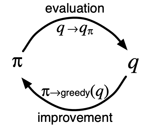
4.6 Generalized Policy Iteration
Policy iteration consists of two simultaneous, interacting processes, one making the value function consistent with the current policy (policy evaluation), and the other making the policy greedy with respect to the current value function (policy improvement).
These two processes alternate until hopefully the processes update all states, converging on the optimal value function and policy.
The term generalized policy iteration (GPI) refers to this idea of interaction between evaluation and improvement. If both evaluation and improvement stabilize, i.e. no longer produce changes, the the value function and optimal policy must be optimal.
Thus, both processes stabilize only when a policy has been found that is greedy with respect to its own evaluation function.
4.7 Efficiency of Dynamic Programming
While DP may not be practical for very large programs, they're relatively efficient for solving MDPs. In the worst case, ignoring some technical details, DP methods take polynomial time to find an optimal policy. If represent the states and actions, then a DP method is guaranteed to find an optimal policy in deterministic time.
On problems with large state spaces, asynchronous DP methods are often preferred.
4.8 Summary
Policy evaluation and policy improvement typically refer to the iterative computation of the value functions for a given policy and the improvement of that policy given the value function of its prior self, respectively.
Combined, these two terms yield policy iteration and value iteration refer to the two most popular DP methods which reliably computer optimal policies and value functions for finite MDPs, given complete knowledge of the MDP.
Class DP methods operate in sweeps through a state set, performing full backup operation on each state, updating the value of the state based on the values of all weighted possibilities of the values of successor states. These are related to Bellman equationsL there are four primary value functions () corresponding to four Bellman equations and their full backups.
Generalized Policy Iteration is the general idea of two interacting processes revolving around approximate policies and value functions is that each process changes the basis for the other, overall working towards a convergent, joint solution where each, consequently, is optimal.
Note that all DP methods update estimates of the values of states based on the estimates of the values of successor states, which is called bootstrapping.
Chapter 5: Monte Carlo Methods
Monte Carlo methods require only experience composed of sample sequences of states, actions, and rewards from interaction with the environment. To ensure well-defined returns, we define Monte Carlo methods only for episodic tasks and only calculate value estimates and policies updates after episodes have terminated.
Monte Carlo methods can thus be incremental in an episode-by-episode sense, but not in a step-by-step (online) sense... Here we use it specifically for methods based on averaging complete returns (as opposed to methods that learn from partial returns, considered in the next chapter).
Monte Carlo methods sample average returns for state-action pairs like the bandit methods sampled average rewards previously - the difference being each state represents a bandit problem and are interrelated to one another. Thus, the problems are nonstationary.
To handle this nonstationary component of practical RL contexts, we adapt the General Policy Iteration techniques from CH 4 where we computed value functions to learning value functions from sample returns of an MDP.
First we consider the prediction problem (the computation of and for a fixed arbitrary policy ) then policy improvement, and, finally, the control problem and its solution by GPI. Each of these ideas taken from DP is extended to the Monte Carlo case in which only sample experience is available
5.1 Monte Carlo Prediction
Recall that the value of a state is the expected return—expected cumulative future discounted reward—starting from that state. An obvious way to estimate it from experience, then, is simply to average the returns observed after visits to that state. As more returns are observed, the average should converge to the expected value.
The first-visit to a state under a Monte Carlo method estimates , and theevery-visit Monte Carlo method averages returns from all states.
First Visit MC Method
Note that we use capital for the approximate value function as it becomes a random variable after initialization.
Both first- and every-visit MC methods converge to as the number of visits to goes to infinity and each return is an independent, identically distributed estimate of with infinite variance.Each averaged is an unbiased estimate with , where is the number of returns averaged. Every-visit is more complicated, but its estimates also asymptotically converge to .
For the given example of blackjack, MC methods are superior to strict DP as DP methods require the distribution of next events (given by ), and those are difficult to determine in a game of blackjack as defined in the example.
An important fact about Monte Carlo methods is that the estimates for each state are independent. The estimate for one state does not build upon the estimate of any other state, as is the case in DP. In other words, Monte Carlo methods do not bootstrap as we defined it in the previous chapter... In particular, note that the computational expense of estimating the value of a single state is independent of the number of states. This can make Monte Carlo methods particularly attractive when one requires the value of only one or a subset of states. One can generate many sample episodes starting from the states of interest, averaging returns from only these states ignoring all others. This is a third advantage Monte Carlo methods can have over DP methods (after the ability to learn from actual experience and from simulated experience).
5.2 Monte Carlo Estimation of Action Values
If a model is not available, then it is particularly useful to estimate action values (the values of state–action pairs) rather than state values.
With a model, state values alone would be sufficient to determine an optimal policy by choosing the action that leads to the best combination of reward and . Without a model, state values alone are insufficient as you must explicitly estimate the value of each action order for the values to be useful in suggesting a policy.
Thus, one of our primary goals for Monte Carlo methods is to estimate . To achieve this, we first consider the policy evaluation problem for action values
Similarly, the evaluation problem for action values is to estimate : the expected return starting from , taking action , and following thereafter. We simply modify the MC method to handle state-action pairs rather than only the states. Just as before, these MC methods converge quadratically upon the expected values as the number of visits to all state-action pairs approaches infinity.
Difficulties arise as many state-action pairs may never be visited. If is deterministic, then following it will observe returns only for one of the actions from each state. The no returns from the missing actions, the MC estimates of those will not improve with experience. This hinders the intentional ability to compare estimated values of all actions from each state.
This is similar to the exploration/exploitation problem insofar as we have to maintain exploration and can be resolved by specifying that episodes start in a state-action pair, and that each pair has a nonzero probability of being selected as the start. This ensures that all state-action pairs will be visited ad infinitum eventually - this is called the assumption of exploring starts.
5.3 Monte Carlo Control
MC Control refers to using MC estimation to approximate optimal policies.
The value function is repeatedly altered to more closely approximate the value function for the current policy, and the policy is repeatedly improved with respect to the current value function:

While each of these improvement and evaluation arcs work against one another by creating moving targets, they effectively force the policy and value function to approach optimality.
Again, we'll use the diagram:
to understand the process. Under the assumptions of infinite episodes generated with exploring starts, MC methods will compute each for arbitrary .
Policy improvement is achieved by making the policy greedy w.r.t the current value function. For any action-value function , the corresponding greedy poly is the one that deterministically chooses an action the the maximal action-value:
The corresponding policy improvement can be achieved by constructing each as the greedy policy w.r.t. . Using the policy improvement theorem from CH 4.2:
As discussed in Chapter 4, this theorem ensures that each is uniformly as good, if not better than : they will both be optimal policies.
This theorem holds so long as the shaky assumptions of exploratory starts and policy evaluation performed over infinite episodes hold...
To obtain a practical algorithm we will have to remove both assumptions.
woot. Let's deal with the first assumption which is relatively easy to remove (can't wait to fix the 2nd assumption). There are two possible solutions: hold firm the idea of approximating in each policy evaluation, and the other is to forgo complete policy evaluation before returning to improvement.
For MC policy evaluation, it is common to episodically alternate between evaluation and improvement: after each episode, the observed returns are used for policy evaluation, and then the policy is improved at all the states visited in the episode:
Under an exploratory start, all returns for each state-action pair are accumulated and averaged, regardless of what policy they were earned under. This implies that an MS ES cannot converge to any sub-optimal policy, otherwise the value function would eventually converge to the value function for that bad policy, forcing a change in the policy.
Convergence to this optimal fixed point seems inevitable as the changes to the action-value function decrease over time, but has not yet been formally proved.
5.4 Monte Carlo Control Without Exploring Starts
The two general approaches to avoid the unlikely assumption of exploring starts is –to ensure that all actions are selected infinitely often– are called on-policy and off-policy methods.
On policy methods attempt to evaluate or improve the policy that is used to make decisions, whereas off-policy methods evaluate or improve a policy different from that used to generate the data.
In on-policy control methods, the policy is soft, meaning that , but gradually shifted closer to a deterministic optimal policy. We can use ε-greedy, or ε-soft exploration to achieve this.
The overall idea of on-policy Monte Carlo control is still that of GPI. As in Monte Carlo ES, we use first-visit MC methods to estimate the action-value function for the current policy.
However, we modify the approach the approach so that the policy is ε-greedy as we do not have the benefit of ES and still need to ensure exploration. GPI does not require that a policy be taken all the way to a greedy policy, just that it moves toward a greedy policy.
For any ε-soft policy, , any ε-greedy policy with respect to is guaranteed to be better than or equal to .
This is ensured by the policy improvement theorem:
We now prove that equality can hold only when both and are optimal among the ε-soft policies, that is, when they are better than or equal to all other ε-soft policies.
Consider a new environment that is just like the original environment, except with the requirement that policies be ε-soft “moved inside” the environment. The new environment has the same action and state set as the original and behaves as follows. If in state s and taking action a, then with probability the new environment behaves exactly like the old environment. With probability it re-picks the action at random, with equal probabilities, and then behaves like the old environment with the new, random action. The best one can do in this new environment with general policies is the same as the best one could do in the original environment with ε-soft policies. Let and denote the optimal value functions for the new environment. Then a policy is optimal among ε-soft policies if and only if . From the definition of we know that it is the unique solution to
Which is identical to the above equation with substituted for ; since is the unique solution, it must be that .
In sum, this shows that policy improvement works for ε-soft policies.
This analysis is independent of how the action-value functions are determined at each stage, but it does assume that they are computed exactly.
The full algorithm for an ε-soft soft policy is given by:
5.5 Off-policy Prediction via Importance Sampling
So far we have considered methods for estimating the value functions for a policy given an infinite supply of episodes generated using that policy. Suppose now that all we have are episodes generated from a different policy. That is, suppose we wish to estimate or , but all we have are episode following another policy .
Here, is the target policy and is the behavior policy. The goal and challenge of off-policy learning is learning about a policy given only episodic experience from no that policy.
In order to meaningfully learn from , we must ensure that every action taken under is also taken, at least occasionally, under : . This is called the assumption of coverage: . Thus must be stochastic in states where it is not identical to , although the target can be deterministic.
Importance Sampling is the general technique used for estimating expected values under one distribution () given samples from another (). Given a starting state , the probability of the subsequent state-action trajectory, , occurring under any policy is:
, where is the state-transition probability function.
Thus, the relative probability of the trajectory under the target and behavior policies (the Importance Sampling Ration) is:
Note that although the trajectory probabilities depend on the MDP’s transition probabilities, which are generally unknown, all the transition probabilities cancel and drop out. The importance sampling ratio ends up depending only on the two policies and not at all on the MDP.
When applying off-ploicy importance sampling to a MC method, it is convenient to number the time steps that increases across episode boundaries s.t. the first episode ends at and the second begins at . We can define the set of all time steps in which is visited as . e.g. for a first-visit method, would only include time steps that were first visits to in their episode. We'll also let by the first time of termination following to denote the return after through . Therefore, , are the returns pertaining to state , and the corresponding importance-sampling ratios. Using these to estimate , we and average the returns scaled by the ratios:
When performed as a simple average as above, this method is called Ordinary Importance Sampling. Alternatively, we can refine value and increase the speed of convergence towards an optimal policy by using a Weighted Importance Sampling:
(accounting for division by 0 making the whole term 0).
Formally, the difference between the two kinds of importance sampling is expressed in their variances. The variance of the ordinary importance sampling estimator is in general unbounded because the variance of the ratios is unbounded, whereas in the weighted estimator the largest weight on any single return is one.
We can verify that the variance of importance-sampling-scaled returns is infinite:
Meaning our variance is only infinite if the expectation of the square of the random variable is infinite.
5.6 Incremental Implementation
Monte Carlo prediction methods can be implemented incrementally, on an episode-by-episode basis, using extensions of the techniques described in Chapter 2. Whereas in Chapter 2 we averaged rewards, in Monte Carlo methods we average returns. In all other respects exactly the same methods as used in Chapter 2 can be used for on-policy Monte Carlo methods. For off-policy Monte Carlo methods, we need to separately consider those that use ordinary importance sampling and those that use weighted importance sampling.
We only have to handle the case of off-policy methods using weighted importance sampling. Suppose we have a sequence of returns , all starting from the same state with corresponding random weight . We want to estimate:
In order to maintain the cumulative sum of the weights given to the first returns for each state, the update rule for :
Off-policy Monte Carlo Policy Evaluation
Note that this algorithm also work for on-policy evaluation by choosing the target and behavior policies to be the same.
5.7 Off-Policy Monte Carlo Control
Recall that the distinguishing feature of on-policy methods is that they estimate the value of a policy while using it for control. In off-policy methods these two functions are separated. The policy used to generate behavior, called the behavior policy, may in fact be unrelated to the policy that is evaluated and improved, called the target policy. An advantage of this separation is that the target policy may be deterministic (e.g., greedy), while the behavior policy can continue to sample all possible actions.
Recall that these techniques requires that the behavior policy has a nonzero probability of selecting all actions that might be selected by the target policy under the assumption of coverage and that we that in order to explore all possibilities, we require that the behavior policy be soft i.e. it selects all actions in all states with nonzero probability.
The following algorithm shows an off-policy Monte Carlo method, based on GPI and weighted importance sampling, for estimating . The target policy is the greedy policy with respect to , which is an estimate of . The behavior policy can be anything, but in order to assure convergence of to the optimal policy, an infinite number of returns must be obtained for each pair of state and action. This can be assured by choosing to be -soft.
Off-policy Monte Carlo GPI with Weighted Importance Sampling to Estimate
However, this method only learns from the tails of episodes, after learning the last nongreedy action, so if those are frequent, learning will be slow, especially for states at the beginning of long episodes. This can be resolved with TD learning covered in the next chapter, or by ensuring that
5.8 Importance Sampling on Truncated Returns
In cases where discounted returns are 0 as , the ordinary importance sampling will be called by the entire product, even if the last 99 factors are zero. These 0 terms are irrelevant to the expected return of a policy, but enormously contribute to the variance (in some cases making it infinite). We can avoid this by thinking of discounting as determining a probability of termination, or a degree of partial termination. For any , we can think of the return as partly terminating in one step, to the degree , producing a return of just the first reward ; partly terminating after two steps to the degree yielding return of ; so on. The partial Each refers to the termination not occurring in any of the prior steps. The partial returns here are called flat partial returns:
where "flat" denotes the absence of discounting, and "partial" denotes that these returns do not extend all the way to termination, but instead stop at the horizon . The conventional full return can be viewed as a sum of flat partial returns as suggested above as follows:
In order to scale the flat partial returns by an importance sampling ratio that is also truncated, we define ordinary and weighted importance-sampling estimator analogous to those presented in 5.4, 5.5:
5.9 Summary
MC methods presented in this chapter learn optimal value functions and policies from episodic experience sampling. This gives (at least) 3 advantages over DP methods:
They can learn optimal behavior directly from interaction with the environment without a model of environment dynamics,
The can be used with simulation or sample models without explicit models of transition dynamics required by DP methods,
MC methods can focus on small subsets of states to learn regions of special interest.
MC methods follow a similar GPI process presented in Chapter 4, with the difference being evaluation of returns from a start state rather than computing values for each state from a model. MC methods focus on state-action values rather than state values alone, intermixing evaluation and improvement steps.
The issue of maintaining sufficient exploration is resolved by assuming that episodes begin with state-action pairs randomly selected over all possibilities.
On-policy methods commit to exploring and trying to find the best policy that still explores, whereas off-policy methods learn a deterministic optimal policy that may be unrelated to the policy being followed. Off-policy prediction refers to learning the value of a target policy from data generated by a distinct behavior policy based on importance sampling.
Ordinary importance sampling uses a simple average of weighted returns, and produces unbiased estimates but runs the risk of larger, potentially infinite, variance,
Weighted importance sampling uses a weighted average and ensures finite variance (it's typically better).
Chapter 6 Temporal-Difference Learning
Temporal-difference learning (TD) is the combination of Monte Carlo methods and dynamic programming. Drawing from model-free, raw experience sample, TDL is similar to MC methods; like DP, TD methods update estimates based in part on other estimates.
6.1 TD Prediction
Just as before with previously examined means of GPI, given some experience following a policy , TD will updates its estimate of for non terminal states . MC methods wait until the return following the visit is known, then use that return as the target for . A simple every-visit MC method suitable for nonstationary environments is:
where is the actual return following time , and is a constant step-size parameter: constant-α MC.
Whereas Monte Carlo methods must wait until the end of the episode to determine the increment to (only then is known), TD methods need wait only until the next time step. At time they immediately form a target and make a useful update using the observed reward and the estimate .
The simplest TD method, , is given by:
Whereas the target for the MC update is , the TD target update is . Because TD methods base their updates in part on an existing estimate, we can adapt the derivation from the DP policy value from CH3:
Whereas MC methods use the first of the last two equation as the target, DP methods use a sampled estimate of the latter.
We call these sample backups because they involve looking ahead to a sample successor state (or state-action pair), using the value of the successor and the reward along the way to compute a backed-up value, and then changing the value of the original state accordingly.
Besides giving you something to do while waiting in traffic, there are several computational reasons why it is advantageous to learn based on your current predictions rather than waiting until termination when you know the actual return.
6.2 Advantages of TD Prediction Models
TD methods learn their estimates in part on the basis of other estimates. They learn a guess from a guess — they bootstrap.
Advantages of TD methods over DP and MC methods include:
they do not require a model of the environment, its rewards, or the next-state probability distributions, unlike DP methods which do;
they are naturally implemented in an online, fully incremental fashion, unlike MC methods where one must wait till the end of an episode when the return is known. TD methods only need a single time step;
MC methods must ignore or discount episodes during which experimental actions are taken, which drastically slows learning.
On top of all that, TD methods are still guaranteed to converge. The natural question that follows is: which method, TD or MC, will converge faster, as they both asymptotically approach correct predictions? As of 2014,-2017, This is an open question, dab.
6.3 Optimality of
Even without limited (non-infinite) experiences, incremental learning can converge on a solution by repeatedly training on the available experiences.
Given an approximate value function, V , the increments specified by previous chapters are computed for every time step at which a non-terminal state is visited, but the value function is changed only once, by the sum of all the increments. Then all the available experience is processed again with the new value function to produce a new overall increment, and so on, until the value function converges. We call this batch updating because updates are made only after processing each complete batch of training data.
converges deterministically under batch training with sufficiently small step-size parameter . A constant-α MC method also converges deterministically, but to a different answer. This is illustrated by example exercises 6.3, 6.4. The conclusion is that Batch MC methods always find the estimates that minimize MSA on the training set, whereas always finds the estimates that would be exactly correct for the maximum-likelihood model of the MDP, where the maximum-likelihood estimate of a parameter is the parameter value whose probability of generating the data is greatest. A certainty-equivalence estimate is the estimate of the value function that would be exactly correct if the model were exactly correct. converges to the former, and therefore converge (with batch training) to a solution faster than MC methods. Without batch training, TD methods do not achieve certainty-equivalence or MSE estimates, but roughly approach them.
6.4 Sarsa: On-Policy TD Control
Now examine the use of TD prediction for the control problem following the GPI pattern. As with MC methods, we need to address the exploration problem for on- and off-policy control methods.
The first step is to learn an action-value function rather than the state-value function. Whereas we'd previously consider the transitions between states, we no consider the transitions from state-action pairs to state-action pars, learning their respective values. Formally these cases are identical MDPs with reward processes, so we know that they are convergent.
On-policy TD Control Algorithm
The update is performed after every transition from a nonterminal state . If is terminal, then is defined to be zero. Thus uses every element of the quintuple of events which gives rise to the name Sarsa.
It is straightforward to design an on-policy control algorithm based on the Sarsa prediction method. As in all on-policy methods, we continually estimate for the behavior policy , and at the same time change toward greediness with respect to .
6.5 Q-Learning: Off-Policy TD Control
Praise be to Watkins, 1989 for Q-Learning in its simplest form given by:
Here, directly approximates , regardless of the policy being followed. This dramatically simplifies the analysis of the algorithm and enables early convergence proofs. All that is required for correct convergence is that all pairs continue to be updated.
Q-Learning: An Off-policy TD Control Algorithm
Example 6.6 compares Sarsa to Q-Learning.
6.6 Games, Afterstates, and Other Special Cases
State-action values collected for a value function after an agent has acted, like in a game of tic-tac-toe, are called afterstates. Afterstates are useful when we have knowledge of an initial part of the environment's dynamics, but not necessarily the full dynamics. We know typically know the immediate effects of our moves, but not necessarily how our opponent will reply. Afterstate value functions are a natural way to take advantage of this kind of knowledge and produce more efficient learning methods as different actions in different states can still lead to the same state.
6.7 Summary
TD methods are alternatives to MC methods for solving the prediction problem. In their use for GPI, two processes are applied, one to accurately predict returns for the current policy and another to drive local policy improvement. When the first process is based on experience, we must ensure that sufficient exploration occurs which cab be resolved via on- and off-policy methods. Sarsa and (some) Actor-Critic methods are on-policy whereas Q-Learning and R-Learning are off-policy.
The methods presented can be applied online with minimal computation, can be completely expressed via a single equation, and can be implemented with minimal effort.
TD methods can also be applied more generally outside of RL for other types of prediction.
Chapter 7: Eligibility Traces
Eligibility traces can be combined with almost any TD method (like Sarsa and Q-Learning) in order to obtain a general method that may learn more efficiently.
The theoretical view of eligibility is that they are a bridge from TD to MC methods:
When TD methods are augmented with eligibility traces, they produce a family of methods spanning a spectrum that has Monte Carlo methods at one end and one-step TD methods at the other
The mechanical interpretation is that an ET is a temporary record of the occurrence of an event (like taking an action or visiting a state), marking the parameters associated with the event as eligible for undergoing learning changes.
When a TD error occurs, only the eligible states or actions are assigned credit or blame for the error. Thus, eligibility traces help bridge the gap between events and training information. Like TD methods themselves, eligibility traces are a basic mechanism for temporal credit assignment.
These are respectively called the forward and backward views of ET.
The forward view is most useful for understanding what is computed by methods using eligibility traces, whereas the backward view is more appropriate for developing intuition about the algorithms themselves.
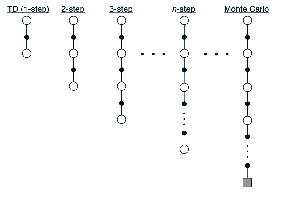
7.1 -Step TD Prediction
Consider estimating from sample episodes generated using . Monte Carlo methods perform a backup for each state based on the entire sequence of observed rewards from that state until the end of the episode. The backup of simple TD methods, on the other hand, is based on just the one next reward,using the value of the state one step later as a proxy for the remaining rewards.
An intermediate approach might perform a backup based on an intermediate amount of rewards. Whereas the TD methods of the previous chapter might backup using the immediate following reward (), until-termination MC would backup based on all rewards ().

In MC methods we backup the estimates of with:
, which we'll call the target of the backup.
A one-step backup target is the first reward plus the discounted estimated reward of the next state:
.
This expression holds for subsequent n-step backups as well, relying on future estimate of at time .
Notationally, it is useful to retain full generality for the correction term. We define the general -step return as:
where in a scalar correction and is called the horizon.
If the episode ends before the horizon is reached, then the truncation effectively occurs at the episode's end, resulting in conventional return s.t. if then , which allows us to treat MC methods as the special case of infinite-step targets.
An -step backup is defined to be a backup toward the -step return. In the tabular, state-value case, the -step backup at time produces the following increment in the estimated value :
, where is a positive step-size parameter, as usual, and increments to estimated values of the other states are defined to be zero.
We define the -step backup in terms of an increment, rather than as a direct update rule as we did in the previous chapter, in order to allow different ways of making the updates. In on-line updating, the updates are made during the episode, as soon as the increment is computed:
, previous chapters have assumed on-line updating.
Off-line updating accumulates increments "on the side" and are not applied to estimates until the end of an episode: does not change during an episode and can simply be denoted . When an episode terminates, the new value for the next episode is obtained by taking the sum of all the increments accumulated during the episode:
With of the following episode being equal to of the current one. We can also apply similar batch updating methods mentioned in 6.3 to. Similarly, optimality of -step returns using are guaranteed to be a better estimate of than . That is to say that the worst error under a new estimate is guaranteed to be less than or equal to times the worst error under :
This is called the error reduction property of -step returns, and can be used to formally prove that on- and off-line TD prediction methods using -step backups converge to the correct predictions under appropriate technical conditions.
Despite this, -step TD methods are rarely used because they suck to implement. Computing their returns requires waiting steps to observe the resultant rewards and states, which very quickly becomes problematic. This is mostly theoretical fluff. Anyways heres Wonderwall Example 7.1 where you're gonna do it anyway lol.
7.2 The Forward View of
-step returns can be average for any amount as long as the weights on the component returns are positive and sum to 1. A backup that averages simpler component backups is called a complex backup. The can be understood as one way of averaging -step backups, each weighted proportional to and normalized by a factor of to ensure summation to 1. The resulting backup towards a return is called the -return:
Here, the on-step return is given the largest weight which is reduced by for each subsequent time step. After a terminal state is reach, all subsequent returns are equal to which can be separated from the main sum as:
This shows that when the main sum goes to zero, and the remaining term reduces to the conventional return . Thus backing up according to the -return is the same as a constant-α MC method from 6.1. Conversely, if , backing up according to the -return yields the one-step return from in 6.2.
The -return algorithm performs backups towards the target. At each step , it computes an increment
.
The overall perfomance of -return algorithms is comparable to that of the -step algorithms. These fall under the theoretical, forward view of a learning alg.
For each state visited, we look forward in time to all the future rewards and decide how best to combine them. After looking forward from and updating one state, we move on to the next and never have to work with the preceding state again. Future states, on the other hand, are viewed and processed repeatedly, once from each vantage point preceding them.
7.3 The Backward View of
This section defines mechanistically to show that it can closely approximate the forward view. The backward view is useful because it is simple both computationally and conceptually. Whereas the forward view is not directly implementable because it is a causal, using at each step knowledge of what will happen many steps later, the backwards view provides a causal, incremental mechanism for approximating the forward view. In the online case, it achieves the forward view exactly.
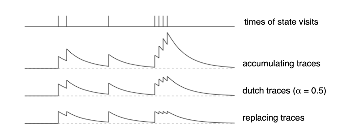
In the backward view of , there is an additional memory variable associated with each state: the eligibility trace, denoted as a random variable . On each step, the eligibility traces of all non-visited states decay by :
, where is the discount rate, and becomes a trace-decay parameter.
For the state visited at time m it also decays, but is incremented:
.
This kind of eligibility trace is called an accumulating trace because it accumulates each time the state is visited, then fades away gradually when the state is not visited
- Eligibility traces keep a simple record of which states have recently been visited, where recency is in terms of . The traces are said to indicate the degree to which each state is eligible for undergoing learning changes should a reinforcing event occur. Reinforcement events such as the moment-by-moment one-step RD errors, like state-value prediction error:
In the backward view of , the global TD error signal triggers proportional updates to all recently visited states, as signaled by their nonzero traces:
These increments could be done at on each step to form an on-line algorithm like the one given below, or saved to the end of an episode to perform an off-line algorithm.
On-line Tabular
The backward view of is aptly oriented backward in time. At each moment, we look at the current TD error and assign it backward to each prior state according to the state's eligibility trace at that time.
Consider what happens at various values of . For , all traces are zero at except for the trace corresponding to . Thus the update reduces to the simple TD rule from 6.2: . For larger values of , more preceeding states behind are changed, but each more temporally distant state is changed less because of the smaller magnitude of its legibility trace. They're given less credit for contributing to the current TD error.
if , then the credit given to the earlier states falls only by per step which matches MC behavior.
Two alternative variations of eligibility traces have been purposed to address limitations of accumulating trace (caused by poor hyper-parameter tuning). On each step, all three trace types decay the traces of the non-visited state in the same way according to , but they differ in how the visited state is incremented. The first variation is the replacing trace which caps the eligibility to 1 whereas accumulation allows for larger values. The second variation is the dutch trace which is an intermediate between the first tow, depending on the step-size parameter :
as approaches zero, the dutch trace mirrors the accumulating trace, and if it approaches 1, it become the replacing trace.

7.4 Equivalences of Forward and Backward Views
Although disparate in origin, both views produce identical value function for all time steps.
True Online is define by the dutch trace with the following value function update:
,
where is an identity-indicator function:
Tabular true on-line
7.5 Sarsa()
This chapter explores how eligibility traces can be used for control, rather than simply prediction as in by combining them with sarsa to produce an on-policy TD control method. As usual, the primary approach is to learn action values rather than state values .
The idea in Sarsa() is to apply the prediction method to state–action pairs rather than to states. Obviously, the, we need a trace not just for each state, but for each state-action pair.
We can the redefine our three types of traces as follows:
Otherwise Sarsa() is just like , substituting state-action variables for state variables: for and for s.t.
Both one-step Sarsa and Sarsa() are on-policy algorithms, meaning that they approximate , the action values for the current policy then improve the policy gradually based on the approximate values for the current policy.
Tabular Sarsa()
7.6 Watkin's Q()
Chris Watkin's, the initial author of Q-learning, also proposed a simple way to combine it with eligibility traces.
Recall that Q-learning is off-policy, meaning that the policy learned about need not be the same as the one used to select actions.
Because Q-learning typically takes exploratory actions (under an ε-greedy policy), special care must be taken when introducing eligibility traces in order to ensure that -step returns bear relationship to the greedy policy.
Unlike or Sarsa(), Watkin's Q() does not look ahead all the way to the end of the episode in it's backup, only as far aheaf as the next exploratory action. Lookahead for each of these algorithms ceases at episode termination otherwise.
The mechanistic, backward view of Watkins's Q() is very simple. Eligibility traces are used just as in Sarsa(), except that they are set to zero whenever an exploratory (non-greedy) action is taken. First, the traces for all state-action pairs are either decayed by or, if an exploratory action was taken, set to 0. Second, the trace corresponding to the current state and action is incremented by 1:
Analagous dutch or replacing traces can also be used here, and the rest of the algorithm is defined by:
,
where
Unfortunately, cutting off traces every time an exploratory action is taken loses much of the advantage of using eligibility traces. If exploratory actions are frequent, as they often are early in learning, then only rarely will backups of more than one or two steps be done, and learning may be little faster than one-step Q-learning.
Tabular Watkin's Q()
7.7 Off-policy Eligibility Traces using Importance Sampling
The eligibility traces from the previous chapter represent a crude way to deal with off-policy training (do my mans Watkin dirty, oh king Sutton) as they treat off-policy as binary –either the target policy is followed and traces continue normally, or it is deviated from and traces are cut off completely– with nothing in between. But the reality is that the target policy may take different actions with different positive probabilities, as may the behavior policy, in which case following and deviating will be a matter of degree. Similarly to what was discussed in CH 5, we can assign credit to a single action using the ratio of the two probabilities of taking an action, and the product of the ratios to assign credit to a sequence.
Additionally, Watkin's Q() confounds bootstrapping and off-policy deviation. Bootstrapping refers to the degree to which an algorithm builds its estimates from other estimates, like TD and DP, or does not, like MC methods. In TD and Sarsa methods, the hyper-parameter denotes teh degree of bootstrapping with denoting no bootstrapping. The same cannot be said of Q() for, as soon as there is a deviation from the target policy, \lambda cuts the trace and uses its value estimate rather than waiting for the actual rewards. Ideally, we should de-couple bootstrapping from teh off-policy aspect.
7.8 Implementation Issues
In practice, implementations avoid the potential issue of updating every state or state-action pair on every time step on serial computers as typical values of are nearly zero, so in practice very few states actually need to be updated.
7.9 Variable
The -return can be significantly generalized beyond what we have described so far by allowing to vary from step to step, that is, by redefining the trace update as
Applications following this generalization are currently still theoretical, but explorations into applying it e.g. varying as a function of the state: .
The elgibility trace equation above is the backward view of variable s, and the corresponding forward view is a more general definition of the -return:
7.10 Conclusions
Eligibility traces in conjunction with TD errors provide an efficient, incremental way of shifting and choosing between Monte Carlo and TD methods. By making TD methods mor like MC methods, they gain the advantage of less-reliance on bootstrapping.
By adjusting , we can place eligibility trace methods anywhere along a continuum from Monte Carlo to one-step TD methods, with a value somewhere in the middle so as not to degrade performance (by running an MC method)
At the expense of computational requirements, eligibility traces learn significantly faster, particularly with many-step reward delays. Thus, traces are useful when data are scarce and cannot be repeatedly processed, as is often the case in on-line applications.
Chapter 8: Planning and Learning with Tabular Methods
This chapter outlines a unified view of the methods that require a model of the environment (planning), like DP and heuristic search, and model-free methods (learning) like MC and TD methods. Both of these types of methods compute value function and are based on looking ahead to future events, computing back-up values, and using it to update an approximate value function. Just as the previous chapter showed how to seemlessly alternate between MC and TD methods, so to will this chapter show how to blend between planning and learning methods.
8.1 Models and Planning
To recap, a model of the environment is anythign that an agent can use to predict how the environment will respond to its actions based on states, actions, and transition dynamics. If a model is stochastic, then the next possible states and rewards are given by some probability distribution and are thus called distribution models. Sample models produce just one of the possibilites according to the probabilites.
For example, consider modeling the sum of a dozen dice. A distribution model would produce all possible sums and their probabilities of occurring, whereas a sample model would produce an individual sum drawn according to this probability distribution.
Models can be used to simulate experience. i.e. sample model could produce an entire episode, and a distribution model could generate all possible episodes and their probabilities.
Here, planning refers to the computational process to infer or improve a policy from a modeled environment:
In state-space planning, planning is primarily viewed as a search the the state space for an optimal policy. In plan-space planning planning primarily viewed as a search through the space of plans (evolutionary methods and partial-order planning are subsets therein). The latter difficult to apply efficiently to stochastic problems which tend to be the focus in RL.
The unified view presented contends that all state-space planning methods share a common, and familiar structure following 2 basic ideas:
all SSP methods involve computing value functions as a key intermediate step towards policy improvement
they compute value functions by backup operations applied to simulated experience.
DP methods fits this structure by sweeping the state space, generating distributions of possible transitions, then computing backed-up values and updating estimated state values. This chapter covers how other SSP methods also fit this structure.
Learning methods require only experience as input, and can typically be applied to simulated experience just as well as to real experience. The following random-sample one-step tabular Q-planning algorithm converges to the optimal policy for the model under the same conditions that the one-step tabular Q-learning alg converges to the optimal policy for the real environment.
Random-Sample One-step Tabular Q-planning
The second theme covered in this chapter is the benefits of planning in small, incremental steps, which enables planning to be interrupted or redirected at any time with minimal wasted computation. This holds for pure planning problems if the problem is too large to be solved exactly.
8.2 Integrating Planning, Acting, and Learning
When planning is done on-line, while interacting with the environment, a number of interesting issues arise.
New information can change the model and therefore the planning. But, if decision-making and model-learning are both computationally-intensive, then the available resources may need to be divided between them. The first exploration of this issue if Dyna-Q, which integrates the major functions needed in an on-line planning agent. Each function appears in Dyna-Q in a simple form.
Experience plays two roles for experience: model improvement (to make the model more closely match the real environment) and to policy improvement (similar to everything discussed till now).


The use of experience to improve the model is also called indirect reinforcment learning, which makes fuller use of a limited amount of experience and thus achieves a better policy with fewer environmental interactions. Direct methods are much simpler and remain unaffected by the biases in the design of the model.
Dyna-Q involves planning, acting, model-learning, and direct RL, continually. The direct RL method is one-step tabular Q-learning, and the model-learning is also table-based, acting on the presumption of a deterministic environment. During planning, the Q-planning algorithm randomly samples only from state-action pairs that have previously been experienced s.t. the model is never queried about a pair about which it has no informaiton.
Conceptually, planning, acting, model-learning, and direct RL occur simultaneously and in parallel to Dyna agents. For concreteness and implementation on a serial computer, we specify the order in which they occur given by the following algoirhtm.
Dyna-Q Algorithm
where denotes the contents of the model (predicted next state and reward) for a state-action pair.
Without planning (), each episode adds only one additional step to the policy, and so only one step (the last) has been learned so far. With planning, again only one step is learned during the first episode, but here during the second episode an extensive policy has been developed that by the episode’s end will reach almost back to the start state. This policy is built by the planning process while the agent is still wandering near the start state. By the end of the third episode a complete optimal policy will have been found and perfect performance attained.
8.3 When the Model Is Wrong
Models can often be incorrect due to stochasticity, limited samples, imperfect generalization of value function approximation, and changes to the environment that have not yet been observed/added to the model. Luckily, suboptimal policies computed by quick planning typically leads to discovery and correction of modeling error. Whereas changes to the environment for the worse (in terms of the current policy) are detected quickly as described above, changes for the better tned not to reveal improvement, and modeling error may not be corrected ever.
The Dyna-Q+ model corrects for the under re-exploration of previously sub-optimal that cause standard Dyna algs to fail at short-cut tasks (where a the model improves after steps, and the optimal policy changes) as follows:
To encourage behavior that tests long-untried actions, a special “bonus reward” is given on simulated experiences involving these actions. In particular, if the modeled reward for a transition is , and the transition has not been tried in time steps, then planning backups are done as if that transition produced a reward of , for some small .
8.4 Prioritized Sweeping
The Dyna agents presented before simulate transitions starting from state-action pairs selected uniformly at random from all experienced pairs, but this can be improved by prioritizing the distribution.
At the beginning of the second episode, only the state–action pair leading directly into the goal has a positive value; the values of all other pairs are still zero. This means that it is pointless to back up along almost all transitions, because they take the agent from one zero-valued state to another, and thus the backups would have no effect. Only a backup along a transition into the state just prior to the goal, or from it into the goal, will change any values.
This can be resolved by working backwards from goal states towards origin points. Though we don't want to use methods specific to the idea of a "goal state"m we can generalize methods according to reward functions.
Suppose now that the agent discovers a change in the environment and changes its estimated value of one state. Typically, this will imply that the values of many other states should also be changed, but the only useful onestep backups are those of actions that lead directly into the one state whose value has already been changed.
As the set of useful backups propogates backward, growing exponentially, computational demands grow as well. Not all of these backups are useful, relative to how much they've changed.
In a stochastic environment, variations in estimated transition probabilities also contribute to variations in the sizes of changes and in the urgency with which pairs need to be backed up.
Prioritizing based on urgency of change is prioritiziation sweeping. By maintaining a priority queue of all state-action pars whose estimated value would change significantly of backed up, prioritized by the size of the change, effects of changes are efficiently propogated backward until quiescence as given by the following algorithm.
Prioritized Sweeping Algorithm for a Deterministic Algorithm
This kinda sucks though:
the algorithms that have been developed so far appear not to extend easily to more interesting cases.
This is due to the assumptin of discrete states. Extensions of prioritized sweeping to stochastic environments are relatively straightforward by simply tracking the probabilities of future states when backing up
8.5 Full vs. Sample Backups
One-step backups vary along three binary dimensions. The first two are whether or not they back up state-values or action-values and whether they estimate the value of the opimal policy or some arbitrary policy. These gives s the four classes of backups for value functions: . The other dimension is whether the backups are full or sample backups, considering all possible events or a single sample of what might happen. This final dimension gives us possibilities, seven of which have specific algorithms shown below.
(The eighth case does not seem to correspond to any useful backup.)

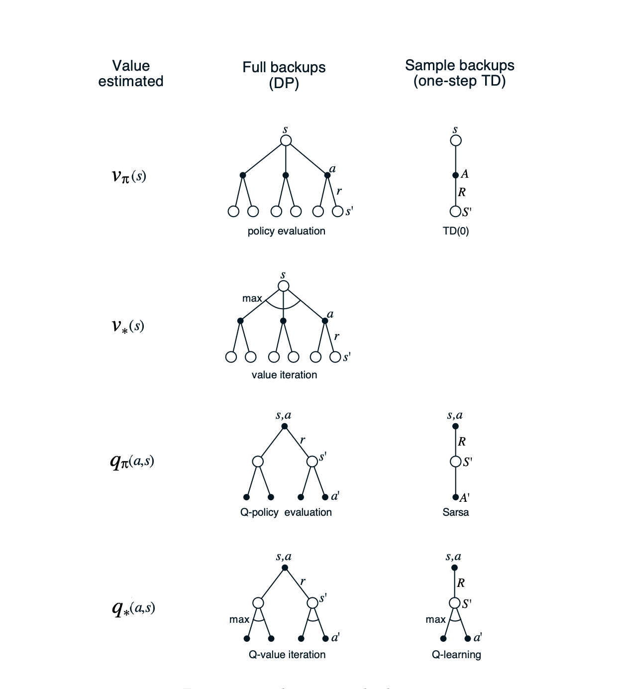
Any of these one-step backups can be used in planning methods. E.g. Dyna-Q used sample backups, but could just as easily have used sample backups ; Dyna-AC used sample backups.
For stochastic problems, prioritized sweeping is always done using one of the full backups.
To determine the merits of full and sample backups, we measure computational requirements.
Consider the following full and sample backups for approximating under discrete states and actions, allowing for tabular representation for , where describes the estimated transition dynamics.
The difference here is significant to the extent that the environment is stochastic.
If there are many possible next states, then there may be significant differences. . In favor of the full backup is that it is an exact computation, resulting in a new whose correctness is limited only by the correctness of the at successor states. The sample backup is in addition affected by sampling error. On the other hand, the sample backup is cheaper computationally because it considers only one next state, not all possible next states.
Let be the starting pair and branching factor (# possible next states that may occur with positive probability), then a full backup requires times as much computation as a sample backup. If there is insufficient time to complete a full backup, sample backups are always prefereable as they at least make some improvement in the value estimate with fewer than backups. Thus the question is: given a unit of computational effort, is it better used on a few full backups or to times as many sample backups?
Analysis suggests that sample backups reduce error according to , where is the number of sampel backups that have been performed (assuming ). The advantage of sample backups is that they cause estimates to get gudder sooner and future estimates from successor states will be more accurate than full backups.
8.6 Trajectory Sampling
The classical approach to distributing backups, from DP, sweeps the entire state or state-action space, backing up each state/state-action pair once. This fails on large tasks due to time constrains. Most of the states visited are irrelevant. A better approach is to sample the space at hand, (preferably smarter than uniformly, rather according to the on-policy distribution). Sample state transitions and rewards are given by the model, simulating explicit individual trajectories and performing backups encountered along the way; this is called trajectory sampling. Following the on-policy distribution is good because it emphasizes states that the agent might actually encounter. Only once stochasticity reaches , does uniform sampling converge towards on-policy sampling performance.
In the short term, sampling according to the on-policy distribution helps by focusing on states that are near descendants of the start state. If there are many states and a small branching factor, this effect will be large and long-lasting. In the long run, focusing on the on-policy distribution may hurt because the commonly occurring states all already have their correct values. Sampling them is useless, whereas sampling other states may actually perform some useful work. This presumably is why the exhaustive, unfocused approach does better in the long run, at least for small problems.
8.7 Heuristic Search
The dominant SSP methods are known as heuristic searches which are conerned with improving action selections given the current value function (rather than other SSP methods which change the value function itself).
In heuristic search, for each state encountered, a large tree of possible continuations is considered. The approximate value function is applied to the leaf nodes and then backed up toward the current state at the root ... The backing up stops at the state–action nodes for the current state. Once the backed-up values of these nodes are computed, the best of them is chosen as the current action, and then all backed-up values are discarded.
Though the value funciton is typically unchanged in heuristic searches, it can be improved over time using backed-up values computed from the search, or any previously discussed methods. Heuristic search is like an extension of the idea of a greedy policy beyond a single step.
If one has a perfect model and an imperfect action-value function, then in fact deeper search will usually yield better policies.
Heuristic search also serves as a means of selectively distributin backups that lead to better and faster approximation of the optimal value function. Just as the search tree is deeper along action trajectories that are more promising and shallower elsewhere, so to can distributions of backups be organized, probably, BSB dunno yet.
The distribution of backups can be altered in similar ways to focus on the current state and its likely successors ... By devoting a large amount of computation specifically relevant to the candidate actions, a much better decision can be made than by relying on unfocused backups.
8.8 Monte Carlo Tree Search
-- chapter missing, TODO, probably also look into 2018 version with SGD
8.9 Summary
This chapter emphasized the relationships between optimal planning and learning behavior, both involving estimating the same value functions, and both updating estimates incrementally.
The most important dimension of variation among SSP methods is the distribution of backups: the focus of the the search.
- Prioritized Sweeping - focuses on the predecessors of states whose values have recently changed
- Heuristic Search - focuses on the successors of the current state
- Trajectory Sampling - focuses on the on-policy distribution
The other dimension explored was the size of the backups.
- smaller backups increase the efficacy of incremental backups
- full backups are just kind of always bad